LLM and Batching: Crucial GPU Optimization in AI

Introduction

In the field of artificial intelligence, GPUs are essential components for processing models, yet their potential is often underutilized. Indeed, these graphics processing units spend a significant amount of time idle between requests. This inefficiency is particularly evident with large language models (LLMs), where the variability of requests can be extreme: some finish in just a few tokens, while others require thousands. This disparity poses a major challenge for traffic management, which must juggle highly uneven workloads.

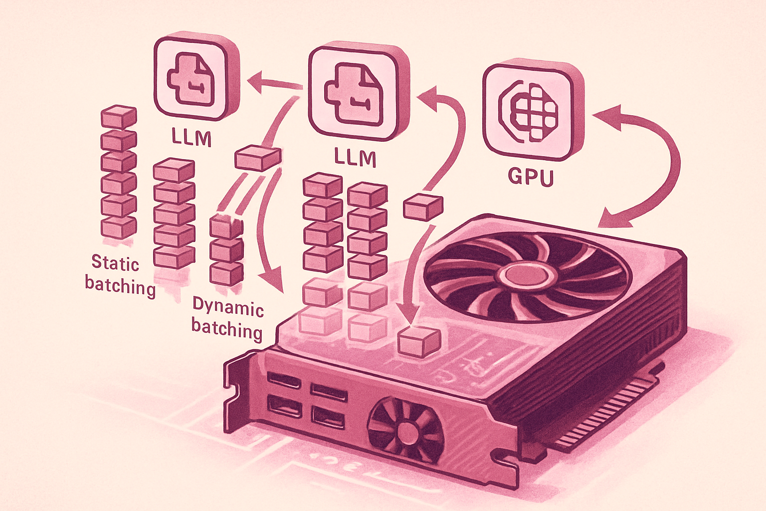
To address this issue, batching emerges as an effective solution. Instead of processing each request individually, batching allows multiple requests to be grouped and executed at once. This transforms the idle cycles of GPUs into useful throughput, optimizing the use of the resources you are already paying for. However, the key to efficiency lies in how these groups are formed, as an inappropriate batching scheme can quickly fail in the face of requests of unpredictable lengths.

How Static Batching Works

Static batching is the most straightforward form of request grouping. It relies on waiting for a fixed number of requests before processing them together. For example, if the batch size is set to eight, the seventh request must wait for an eighth to arrive before processing can begin.

This mechanism is simple: requests accumulate in a queue, and when the number reaches the predefined size, the server executes a single pass over all the requests, sharing a model weight across the group. The main advantage lies in the fact that loading model weights from GPU memory is a costly operation. Doing it once for multiple requests, rather than for each individually, represents a significant efficiency gain. This is why static batching is ideal for scheduled tasks, where latency is not a critical factor.

However, this model has significant limitations for real-time traffic. First, the first request must wait for the batch to be complete, meaning that latency depends on the speed of arrival of other requests. Additionally, once the batch is in progress, all requests must wait for the slowest one to finish, which can delay the entire process. Finally, there is no way to limit the waiting time before a batch begins, making static batching unsuitable for applications requiring low latency.

How Dynamic Batching Works

Dynamic batching takes the principle of grouping requests to share a model weight but eliminates the requirement for a complete group before processing begins. Instead, the server sets two limits: a maximum batch size and a time window. The execution of the batch is triggered as soon as either of these limits is reached.

In practical terms, this means that as soon as the first request arrives, a timer starts. If enough requests arrive to fill the batch before the timer expires, they are processed immediately. Otherwise, the server executes what has been accumulated so far, even if the batch is partial.

An optimized dynamic batching configuration on a Triton inference benchmark has significantly improved throughput while introducing a moderate increase in queue latency. This is a typical trade-off of dynamic batching: increased hardware utilization and higher throughput result in slightly longer response times.

Dynamic batching thus offers increased throughput, and the time window determines the latency you are willing to accept. A shorter window protects latency at the cost of smaller and less efficient batches, while a longer window increases the chances of obtaining a complete batch but extends the waiting time for the first requests.

The maximum batch size still limits the amount of work that can share a model weight, regardless of the time window parameter. However, this method does not solve the problem of long requests blocking the entire batch. For models requiring a variable number of tokens, this means that short requests often wait behind long ones without any possibility of bypass.

How Continuous Batching Works

Continuous batching introduces a radically different approach by replacing the request as the scheduling unit with the individual decoding step. Instead of waiting for the end of each sequence in a batch before starting the next, the server tracks each sequence independently, one token at a time.

During servicing, at each decoding iteration, the server produces the next token for each active sequence simultaneously. As soon as a sequence emits an end token, it is removed from the batch, and a new request is inserted in its place during the next iteration.

In this model, there is no fixed batch to complete. Instead, a rolling set of active sequences changes almost at every step, meaning that a GPU running continuous batching is rarely idle.

A sequence that finishes early immediately frees its slot, rather than delaying the rest of the batch. A new request only needs to wait for a single iteration to be inserted into a free slot, rather than until the end of a complete batch cycle.

The initial pre-filling pass of a new request is computationally heavy and can delay the decoding step for every other active sequence during that iteration. Chunked pre-filling breaks these long prompts into smaller segments, processed over multiple steps.

Continuous batching is also known as in-flight batching in TensorRT-LLM. Many inference frameworks for LLMs, such as vLLM and TGI, favor continuous batching for its ability to deliver high throughput under concurrent workloads. In contrast, dynamic batching at the request level can offer faster time to the first token under light loads.

Summary

The different batching techniques address the same problem with varying levels of granularity. Static batching shares a model weight across a group but imposes a wait for the slowest request. Dynamic batching reduces this wait by adding a time delay but cannot speed up a batch once it has started. Continuous batching completely eliminates the fixed batch, scheduling at the level of individual decoding steps, making it the standard choice for large-scale autoregressive language models.

Here’s a summary of the batching strategies:

• Static Batching: Suitable for offline tasks without latency requirements, but with high idle time between batches.
• Dynamic Batching: Offers a trade-off between throughput and latency, ideal for fixed-length outputs.
• Continuous Batching: Optimizes the servicing of autoregressive LLMs in production, with low idle time and high throughput.

For those looking to delve deeper into the subject, several resources are available, including LLM inference manuals and guides on continuous and dynamic batching.