Regression & MLE: a curve reduces the error to 0.134
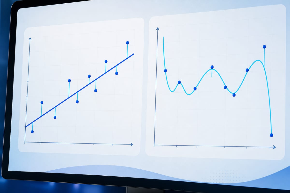
In Regression & MLE, replacing a straight line with a degree 7 curve reduces the displayed error from 0.236 to 0.134, while the curve takes on extreme values at the edges of the graph. The tool allows for comparison of the fit to examples and predictions outside their range.
Predictions Diverge Outside Examples
For the same x-coordinate of 9.9, the line provides 8.461, compared to 14.286 for the curve. The latter fits the available points more closely, but its values become extreme at the ends. At this x-coordinate, which is located beyond the last example, the interface indicates an extrapolation. This alert is a design choice of the tool, not a limitation of the line's ability to recognize its boundaries.
The line deals with coordinates without knowing what they represent. In an example linking study duration and academic results, it would assign a score of 36 out of 10 to 50 hours of study. The calculation would still conform to the model, even if that score makes no sense.
Large models can also apply their parameters to situations where their response loses relevance. An AI tool mobilizes the examples from its training without knowing if the presented case resembles them. A request concerning an atypical client, a new product, or an unusual year can therefore receive a response that appears just as confident as a request for a standard case, despite a result that lacks meaning.
Gray Lines Represent Residuals
The vertical gray lines represent the residuals, in other words, the discrepancies between the observations and the line. To obtain the mean squared error, or MSE, each discrepancy is squared, and then their sum is divided by the number of observations. The squaring prevents discrepancies of opposite signs from canceling each other out and penalizes larger errors more heavily. This method is known as least squares; the loss is the quantity that training seeks to minimize.
After activating the Clear command, clicks allow for the creation of a new set of observations, with a readjustment for each addition. For a single isolated point, an infinite number of lines are suitable, and the MSE equals 0; the software chooses the horizontal line. Two points are also sufficient to achieve an error of 0, since the line passes through them exactly. With the arrival of a third non-aligned point, perfect fitting becomes impossible: the two available parameters are no longer sufficient to pass through all observations.
Le brief IA que les pros lisent chaque soir
Les 7 actus IA du jour, décryptées en 5 min. Gratuit.
Inclus dès l'inscription : notre sélection des meilleurs guides & comparatifs IA.
Choisissez votre rythme
Gratuit · Pas de spam · Désabonnement en 1 clic
With three or four observations, an overfitting alert may appear. The software sequentially excludes each of them, adjusts the line on the others, and then measures the discrepancy on the excluded observation. Such a small set can yield poor results on the unused point; the alert generally disappears with five observations. Another exercise compares the movement of the first point to that of the fifth: an observation located at one end exerts more influence on the line than a central observation.
Two Parameters Summarize Initial Observations
At startup, the graph contains ten observations, each defined by a horizontal coordinate x and a vertical coordinate y. These pairs could link a study duration to a grade, or the area of an apartment to its price. The Reset command restores this initial set.
The line serves as the model here, fully described by its slope and y-intercept. Its initial equation, y = 0.687·x + 1.658, thus contains in these coefficients what the fit has retained from the observations. Searching for these parameters by minimizing the MSE corresponds to the training process. Moving the fifth point upward slightly pivots the line in its direction and increases the error; the coefficients change during the manipulation.
With each movement, a formula directly recalculates the parameters yielding the minimum error. Large models instead proceed through successive corrections of their many parameters, with the same goal of error reduction. Predicting then involves using the model for an x-coordinate absent from the examples: at x = 4, the interface indicates y = 4.407, represented by a green point.
The Origins of Least Squares and Regression
Adrien-Marie Legendre published the method of least squares in 1805. In 1809, Carl Friedrich Gauss stated that he had been using it since 1795.
The term regression, on the other hand, dates back to Francis Galton's research on human height in 1886. He compared the height of children to the average height of their two parents and observed that children had a smaller deviation from the population average. For example, a parental average exceeding this reference by 6 cm corresponded to children exceeding it by about 4 cm.
According to Galton's calculation, children retained about two-thirds of the parental deviation from the average. This tendency to move closer to the average gave its name to regression, without the term implying a backward return.
Brief IA — L'actualité IA en français
L'essentiel de l'actualité de l'intelligence artificielle, décrypté et expliqué chaque jour.