Bayesian Networks: ELBO Makes Approximation Feasible

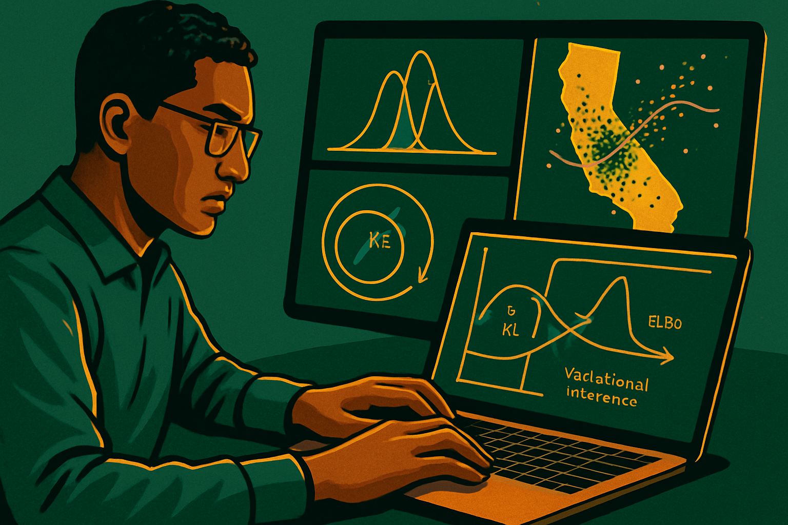
The Bayesian approach promises predictions accompanied by a degree of confidence, but the exact posterior of a network remains out of reach. Variational inference circumvents this obstacle by optimizing an approximation and maximizing the ELBO. Applied to the California Housing dataset, this method provides prediction intervals and concrete safeguards for model usage.

Exact Calculation Impossible, ELBO Guides Approximation

Obtaining the posterior distribution of a network's weights via Bayes' theorem requires calculating p(D), an integral over all combinations of weights. With thousands or millions of parameters, this integration becomes intractable, and the exact answer cannot be computed. In practice, even a few thousand parameters pose a theoretically solvable problem but are too costly in terms of time or memory. Variational inference then reformulates the task into an optimization problem: finding a simpler distribution that resembles the target. It relies on powerful optimization algorithms, proven in high dimensions, to approach otherwise inaccessible distributions. The quality of approximation is traditionally judged by the Kullback–Leibler divergence, which is zero if the distributions coincide and increases otherwise. However, since the target is unknown, the focus is instead on maximizing the ELBO, a computable lower bound derived from the available information. This approach still leaves design choices and training strategies that condition the implementation.

What a Bayesian Network Changes Compared to a Standard Network

A standard network adjusts numerous weights to bring its predictions closer to known outputs and delivers a single answer, without expressing uncertainty. A Bayesian network retains the same architecture but replaces each point weight with a probability distribution, typically Gaussian, although other families are possible. Specifically, a weight is no longer fixed at a value, such as 5.2, but describes a plausible range, for example around 5, between 3 and 7. Some distributions become narrow (when certainty is high), while others are more spread out. After training, a standard network always produces the same output for the same input, while a Bayesian network samples weights at each pass. Thus, repeating the same input generates a collection of outputs from which a prediction interval can be deduced. Where a classical model would announce a median value of $300,000, a Bayesian network might formulate a 95% interval between $250,000 and $350,000.

Epistemic and Random Uncertainty: Practical Utility and Limits

The literature has distinguished since the 17th century between two types of uncertainty: epistemic, related to the model and encountered in configurations never seen before, and random, due to intrinsic variability even for familiar cases. Separating these sources is useful, and some formalisms claim to achieve this, but mathematical definitions sometimes diverge. Recent work suggests that these two dimensions are largely intertwined in machine learning. An operational approach then consists of producing a single uncertainty estimator, without attempting to label the epistemic or random contributions.

California Housing Dataset: 20,640 Rows, 8 Variables, and a Cap at $500,000

The California Housing dataset from scikit-learn, licensed under BSD, is based on the work of Pace and Barry (1997) and derives from the 1990 U.S. Census. The property values it contains do not correspond to the current market. Each observation summarizes a group of census blocks, the smallest sampled geographic unit, encompassing a few hundred to a few thousand people. The dataset describes 20,640 houses through eight variables: median income (MedInc), median age of houses (HouseAge), average rooms per household (AveRooms), average bedrooms (AveBedrms), population, average members per household (AveOccup), latitude, and longitude. The target is the median value per group of blocks. A cap fixes all values above $500,000 at $500,000; for training, all houses valued at $500,000 were removed. A dedicated notebook details the preprocessing and the formation of training and test sets.

Implementation: Weight Distributions, VI, and Uncertainty Bounds

The implementation in Python sets up weight distributions, trains the model through variational inference, and extracts actionable uncertainty bounds to decide when to exploit or discard a prediction. The provided notebooks prioritize uncovering engineering constraints rather than optimizing hyperparameters like layer sizes. Each notebook isolates a design choice to illustrate it. In a production context, it is expected to combine these choices to meet robustness and performance requirements.

Leaving the Illusion of Averages: Beyond MAE and Single Figures

A point prediction, such as a median value of $385,000, may give an impression of precision while obscuring the causes of uncertainty, whether they stem from the data or the model's deviation from an unseen case. Single-output networks do not document this nuance and often only indicate aggregated metrics like MAE, which are not very informative for the present example. A Bayesian framework, on the other hand, aims for a plausible range accompanied by a level of confidence, an approach supported by recent work that encourages integrating uncertainty into automated decisions.