GNN Explained: Understanding and Training a GCN

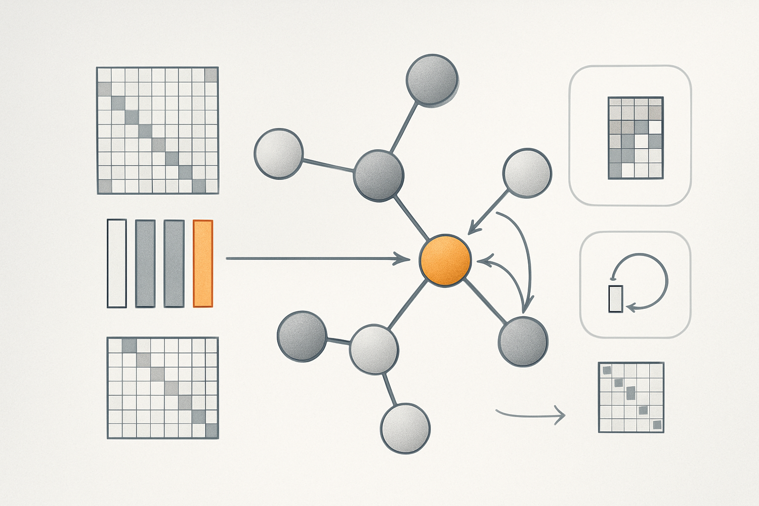
Graph neural networks apply deep learning to relational structures. Their most common variant, the GCN, combines a node and its neighbors to produce new representations. Here’s what these models offer, how they are trained, and the exact way their updates and normalizations are written.

Generalization, Complexity, and Announced Limits

The computations of a GCN are linear with respect to the size of the graph, with a complexity of O(|V| + |E|). Sharing the weight matrix W among the nodes means that the number of parameters does not depend on the size of the input graph. For a given graph structure, GCNs process nodes with different importance based on their proximity to other nodes. GNNs generalize to new structures because they learn transformations applied individually to the nodes. Inference on a new graph generally works well when its structure remains similar to that seen during training; if it differs completely, performance may degrade. Like CNNs, GCNs leverage local context to enhance overall performance. An excessive number of layers is avoided as it can lead to oversmoothing.

Training on One or Multiple Graphs, and Producing Embeddings

Backpropagation in GNNs occurs similarly to that in traditional neural networks. A GNN can be trained on a single large graph or on multiple graphs; generally, training on multiple graphs improves generalization to new graphs. A GNN produces node embeddings, which are then utilized by a separate, smaller model for downstream tasks such as node, edge, or graph classification. In this setup, the labels from the downstream task serve for loss calculation and GNN training. However, there are rare cases where the GNN directly provides the final predictions. The dimension of the feature vectors per layer is a major hyperparameter and can vary between layers.

Updating a GCN Layer Relies on Three Matrices

The update of a GCN layer mobilizes three matrices: A for adjacency, H for node features, and W for the shared learnable linear transformation. In A, A[i][j] equals 1 if vertices i and j are connected and 0 otherwise; the iᵉ row of H encodes the vector of the iᵉ node. The product AH sums the features of neighbors and ignores non-neighbors, then multiplying by W and applying a non-linearity σ provides the updated features. ReLU or LeakyReLU are generally used for σ. By associativity, the computation of AHW is practically done by starting with HW, in order to reduce computational cost by only multiplying by A afterward. Backpropagation progresses from the last layer to the first, while the aggregation of a layer applies in parallel to all nodes. Feature dimensions can change from one layer to another, and the graph structure is preserved across layers.

Including the Central Node and Controlling Scale

In the naive form, a node does not incorporate its own features since A[i][i] equals 0 by default. Adding the identity matrix to A introduces a self-loop that includes the central node in the aggregation and modifies the update rule accordingly. Multiplications alter the scale of features, which motivates normalization by the degree matrix D, where D[i][i] corresponds to the number of neighbors of node i, including the node itself after adding loops, and where D[i][j] equals 0 for i ≠ j. The rule can then be written with this normalization, including as an average at the node level. A common variant applies symmetric normalization by placing D^(−1/2) on both sides of Ā, and is rewritten at the node level via weights depending on the degrees of the nodes (Kipf & Welling, ICLR 2017).

Why Graphs, and What GNNs Inherit from CNNs

Graphs model objects and their relationships in various contexts, including molecules, social networks, players during a match, traffic, or subway maps. Graph neural networks apply deep learning to these structures and, once trained, can be applied to new graphs. They have been used for tasks such as antibiotic discovery and are used to classify nodes, edges, or entire graphs. Their principle borrows from image convolutions: combining an entity with its neighborhood to produce enriched representations. An image can indeed be seen as a graph where a pixel is connected to up to four neighbors. GNNs operate with few layers, typically between 2 and 4, with too high a number potentially causing oversmoothing. Compared to fully connected networks, they learn transformations applied node by node, without linking the number of parameters to the input size. They share with CNNs the exploitation of local context and rely on linear complexity calculations, with a weight matrix shared among all nodes.